Chapter 21
Summarizing and Graphing Survival Data
IN THIS CHAPTER
 Beginning with the basics of survival data
Generating life tables and trying the Kaplan-Meier method
Applying some handy guidelines for survival analysis
Using survival data for even more calculations
This chapter describes statistical techniques that deal with a special kind of numerical data called survival data or time-to-event data. These data reflect the interval from a particular starting point in time, such the date a patient receives a certain diagnosis or undergoes a certain procedure, to the first or only occurrence of a particular kind of event that represents an endpoint. Because these techniques are often applied to situations where the endpoint event is death, we usually call the use of these techniques survival analysis, even when the endpoint is something less drastic (or final) than death. Survival data could include time from resolution of a chronic illness symptom to its relapse, but it can also be a desirable endpoint, such as time to remission of cancer, or time to recovery from an acute condition. Throughout this chapter, we use terms and examples that imply that the endpoint is death, such as saying survival time instead of time to event. However, everything we say also applies to other kinds of endpoints.
You may wonder why you need a special kind of analysis for survival data in the first place. Why not just treat survival times as ordinary numerical variables? Why not summarize them as means, medians, standard deviations, and so on, and graph them as histograms and box-and-whiskers charts? Why not compare survival times between groups with t tests and ANOVAs? Why not use ordinary least-squares regression to explore how various factors influence survival time?
In this chapter, we explain how survival data aren’t like ordinary numerical data and why you need to use specific techniques to analyze them properly. We describe two ways to construct survival curves: the life-table and the Kaplan-Meier methods. We guide you in preparing and interpreting survival curves and show you how to glean useful information from these curves, such as median survival time and five-year survival rates.
Understanding the Basics of Survival Data
To understand survival analysis, you first have to understand survival data. Survival times are intervals between a designated starting time point and the time point an event occurs. These intervals have can have a specific type of missing data due to a phenomenon called censoring. Because survival data usually include censored data, they must be analyzed in a very specific way to avoid generating biased estimates that lead to incorrect conclusions.
Examining how survival times are intervals
The techniques described in this chapter for summarizing, graphing, and comparing survival data deal with the time interval from a defined starting point to the first occurrence of an endpoint event. The event can be designated as death or a relapse of a particular condition, such as a recurrence of cancer. Or you could designate the event to be surgical removal (called an explant) of a failed mechanical component, such as an artificial heart valve. If a patient’s heart valve was implanted on January 10 (beginning of time interval), but their body rejected it and the explant took place on January 30 (time of event), then the time interval from implant to explant is 30 – 10, or 20 days.
A person can die only once, so survival analysis can obviously be used for one-time events. But other endpoints can occur multiple times, such as having a stroke or having cancer go into remission. The techniques we describe in this chapter only analyze time to the first occurrence of the event. More advanced survival analysis methods are needed for models that can handle multiple occurrences of an event, and these are beyond the scope of this book.
 The starting point of the time interval is somewhat arbitrary, so it must be defined explicitly every time you do a survival analysis. Imagine that you’re studying the progression of chronic obstructive pulmonary disease (COPD) in a group of patients. If you want to study the natural history of the disease, the starting point can be the diagnosis date. But if you’re instead interested in evaluating the efficacy of a treatment, the starting point can be defined as the date the treatment began.
Recognizing that survival times aren’t normally distributed
 Even though survival times are numerical quantities, they’re almost never normally distributed. Because of this, it’s generally not a good idea to use the following:
- Means and standard deviations to describe survival times
- T tests and ANOVAs to compare survival times between groups
- Least-squares regression to investigate how survival time is influenced by other factors
If non-normality were the only problem with survival data, you’d be able to summarize survival times as medians and centiles instead of means and standard deviations. Also, you could compare survival between groups with nonparametric Mann-Whitney and Kruskal-Wallis tests instead of t tests and ANOVAs. But time-to-event data are susceptible to a specific type of missingness called censoring. Typical parametric and nonparametric regression methods are not equipped to deal with censoring, so we present survival analysis techniques in this chapter.
Considering censoring
Survival data are defined as the time interval between a selected starting point and an endpoint that represents an event. But unfortunately, the time the event takes place can be missing in survival data. This can happen in two general ways:
- You may not be able to observe all the participants in the data until they have the event. Because of time constraints, at some point, you have to end the study and analyze your data. If your endpoint is death, hopefully at the end of your study, some of the participants are still alive! At that point, you would not know how much longer these participants will ultimately live. You only know that they were still alive up to the last date they were measured in the study as part of data collection, or the last date study staff communicated with them in some way (such as through a follow-up phone call). This date is called the date of last contact or the last-seen date, and would be the date that these participants would be censored in your data.
- You may lose track of some participants during the study. Participants who enroll in a study may be lost to follow-up (LFU), meaning that it is no longer possible for study staff to locate them and continue to collect data for the study. These participants are also censored at their date of last contact, but in the case of LFU, this date is typically well before the observation period ends.
You can describe these two situations in one general way. You know that every participant in the study either died on a certain date (in which case they have the event), or was alive up to some last-seen date when they stopped being observed, in which case they are censored.
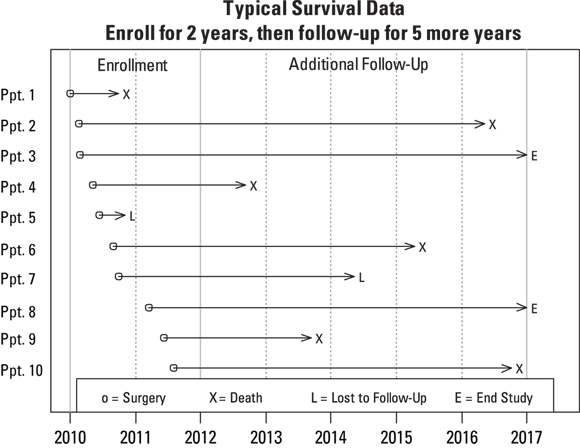
Figure 21-1 shows the results of a small study of survival in cancer patients after a surgical procedure to remove a tumor. Ten patients were recruited to participate in the study and were enrolled at the time of their surgery. The recruitment period went from Jan. 1, 2010, to the end of Dec. 31, 2011 (meaning a two-year enrollment period). All participants were then followed until they died, or until the conclusion of the study, on Dec. 31, 2016, which added five years of additional observation time after the last enrollment. Each participant has a horizontal timeline that starts on the date of surgery and ends with either the date of death or the censoring date.
© John Wiley & Sons, Inc.
FIGURE 21-1: Survival of ten study participants following surgery for cancer.
In Figure 21-1, observe that each line ends with a code, and there’s a legend at the bottom. Six of the ten participants (#’s 1, 2, 4, 6, 9, and 10, labeled X) died during the course of the follow-up study. Two participants (#5 and #7, labeled L) were LFU at some point during the study, and two participants (#3 and #8, labeled E) were still alive at the end of the study. So this study has four participants — the Ls and the Es — with censored survival times.
So, how do you analyze survival data containing censoring? The following sections explain the correct ways to proceed as well as mistakes to avoid.
Analyzing censored data properly
Statisticians have developed techniques to utilize the partial information contained in censored observations. We describe two of the most popular techniques later in this chapter, which are the life-table method and the Kaplan-Meier (K-M) method. To understand these methods, you need to first understand two fundamental concepts — hazard and survival:
- The hazard rate is the probability of the participant dying in the next small interval of time, assuming the participant is alive right now.
- The survival rate is the probability of the participant living for a certain amount of time after some starting time point.
The first task when analyzing survival data is usually to describe how the hazard and survival rates vary with time. In this chapter, we show you how to estimate the hazard and survival rates, summarize them as tables, and display them as graphs. Most of the larger statistical packages (such as those described in Chapter 4) allow you to do the calculations we describe automatically, so you may never have to do them manually. But without first understanding how these methods work, it’s almost impossible to understand any other aspect of survival analysis, so we provide a demonstration for instructional purposes.
Making mistakes with censored data
Here are two mistakes you need to avoid when working with survival data:
- You shouldn’t exclude participants with a censored survival time from any survival analysis!
- You shouldn’t substitute the censored date with some other value, which is called imputing. When you impute numerical data to replace a missing value, it is common to use the last observed value for that participant (called last observation carried forward, or LOCF, imputation). However, you should not impute dates in survival analysis.
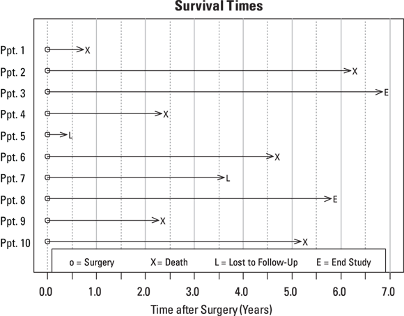
Exclusion and imputation don’t work to fix the missingness in censored data. You can see why in Figure 21-2, where we’ve slid the timelines for all the participants over to the left as if they all had their surgery on the same date. The time scale shows survival time in years after surgery instead of chronological time.
© John Wiley & Sons, Inc.
FIGURE 21-2: Survival times from the date of surgery.
If you exclude all participants who were censored in your analysis, you may be left with analyzable data on too few participants. In this example, there are only six uncensored participants, and removing them would weaken the power of the analysis. Worse, it would also bias the results in subtle and unpredictable ways.
Using the last-seen date in place of the death date for a censored observation may seem like a legitimate use of LOCF imputation, but because the participant did not die during the observation period, it is not acceptable. It’s equivalent to assuming that all censored participants died immediately after the last-contact date. But this assumption isn’t reasonable, because it would not be unusual for them to live on many years. This assumption would also bias your results toward artificially shorter survival times.
 In your analytic data set, only include one variable to represent time observed (such as Time in days, months, or years), and one variable to represent event status (such as Event or Death), coded as 1 if they are have the event during the observation period, and 0 if they are censored. Calculate these variables from raw date variables stored in other parts of the data (such as date of death, date of visit, and so on).
Looking at the Life-Table Method
To estimate survival and hazard rates in a population from a set of observed survival times, some of which are censored, you must combine the information from censored and uncensored observations properly. How is this done? Well, it’s not done by dividing the number of participants alive at a certain time point in the study by the total number of participants in the study, because this fails to account for censored observations.
Instead, think of the observation period in a study as a series of slices of time. Think about how each time a participant survives a slice of time and encounters the next one, they have a certain probability of surviving to the end of that slice and continuing on to encounter the next. The cumulative survival probability can then be obtained by successively multiplying all these individual time-slice survival probabilities together. For example, to survive three years, first the participant has to survive the first slice (Year 1), then survive the second slice (Year 2), and then survive the third slice (Year 3). The probability of surviving all three years is the product of the probabilities of surviving through Year 1, Year 2, and Year 3.
These calculations can be laid out systematically in a life table, which is also called an actuarial life table because of its early use by insurance companies. The calculations only involve addition, subtraction, multiplication, and division, so they can be done manually. They are easy to set up in a spreadsheet format, and there are many life-table templates available for Microsoft Excel and other spreadsheet programs that you can use.
Making a life table
To create a life table from your survival data, you should first break the entire range of survival times into convenient time slices. These can be months, quarters, or years, depending on the time scale of the event you’re studying. Also, you have to consider the time increments in which you want to report your results. You should arrange to have at least five slices or else your survival and hazard estimates will be too coarse to show any useful features. Having many skinny slices doesn’t disturb the calculations, but the life table will have many rows and may become unwieldy. For the survival times shown in Figure 21-2, a natural choice would be to use seven 1-year time slices.
Next, count how many participants experienced the event during each slice, and how many were censored, meaning they were last observed during this time slice and had not experienced the event. From Figure 21-2, you see that
- During the first year after surgery, one participant died (#1), and one participant was censored (#5, who was LFU).
- During the second year, no participants died or were censored.
- During the third year, two participants died (#4 and #9), and none were censored.
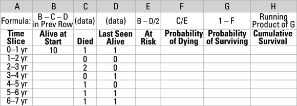
Continue tabulating deaths and censored times for the fourth through seventh years, and enter these counts into the appropriate cells of a spreadsheet like the one shown in Figure 21-3.
© John Wiley & Sons, Inc.
FIGURE 21-3: A partially completed life table to analyze the survival times shown in Figure 21-2.
To fill in the table shown in Figure 21-3:
- Put the description of the time interval that defines each slice into Column A.
- Enter the total number of participants alive at the start into Column B in the 0–1 yr row.
- Enter the counts of participants who died within each time slice into Column C (labeled Died).
- Enter the counts of participants who were censored during each time slice into Column D (labeled Last Seen Alive).
After you’ve entered all the counts, the spreadsheet will look like Figure 21-3. Then you perform the calculations shown in the Formula row at the top of the figure to generate the numbers in all the other cells of the table. (To see what it looks like when the table is completely filled in, take a sneak peek at Figure 21-4.)
Columns B, C, and D
Column B includes the number of participants known to be alive at the start of each year after surgery. This is equal to the number of participants alive at the start of the preceding year minus the number who died (Column C) or were censored (Column D) during the preceding year. Here’s the formula, written in terms of the column letters: B for any year = B – C – D from the preceding year.
Here’s how this process plays out in Figure 21-3:
- Out of the ten participants alive at the start, one died and one was last seen alive during the first year. This means eight participants (10 – 1 – 1) are known to still be alive at the start of the second year. The missing participant is #5, who was LFU during the first year. They are censored and not counted in any subsequent years.
- Zero participants died or were last seen alive during the second year. So, the same eight participants are still known to be alive at the start of the third year.
- Calculations continue the same way for the remaining years.
Column E
Column E shows the number of participants at risk for dying during each year. You may guess that this is the number of participants alive at the start of the interval, but there’s one minor correction. If any were censored during that year, then they weren’t technically able to be observed for the entire year. Though they may die that year, if they are censored before then, the study will miss it. What if you don’t know exactly when during that year they became censored? If you don’t have the exact date, you can consider them being observed for half the time period (in this case, 0.5 years). So the number at risk can be estimated as the number alive at the start of the year, minus one-half of the number who became censored during that year, as indicated by the formula for Column E: E = B – D/2. (Note: To simplify the example, we are using years, but you could use months instead if you have exact censoring and death dates in your data to improve the accuracy of your analysis.)
Here’s how this formula works in Figure 21-3:
- Ten participants were alive at the start of Year 1, and one participant was censored during Year 1. To correct for censoring, divide 1 by 2, which is 0.5. Next, subtract 0.5 from 10 to get 9.5. After correcting for censoring, only 9.5 participants are at risk of dying during Year 1.
- Eight participants were alive at the start of Year 2, and zero were censored during Year 2. So all eight participants continued to be at risk during Year 2.
- Calculations continue in the same way for the remaining years.
Column F
Column F shows the Probability of Dying during each interval, assuming the participant has survived up to the start of that interval. To calculate this, divide the Died column by the At Risk column. This represents the fraction of those who were at risk of dying at the beginning of the interval who actually died during the interval. Formula for Column F: F = C/E.
Here’s how this formula works in Figure 22-3:
- For Year 1, the probability of dying is calculated by dividing the one death by the 9.5 participants at risk: 1/9.5, or 0.105 (10.5 percent).
- Zero participants died in Year 2. So, for participants surviving Year 1 and alive at the beginning of Year 2, the probability of dying during Year 2 is 0. Woo-hoo!
- Calculations continue in the same way for the remaining years.
Column G
Column G shows the Probability of Surviving during each interval for participants who have survived up to the start of that interval. Since surviving means not dying, the equation for this column is 1 – Probability of Dying, as indicated by the formula for Column G: G = 1 – F.
Here’s how this formula works out in Figure 22-3:
- The probability of dying in Year 1 is 0.105, so the probability of surviving in Year 1 is 1 – 0.105, or 0.895.
- The probability of dying in Year 2 is 0.000, so the probability of surviving in Year 2 is 1 – 0.000, or 1.000.
- Calculations continue in the same way for the remaining years.
Column H
Column H shows the cumulative probability of surviving from the time of surgery all the way through the end of this time slice. To survive from the start time through the end of any given year (year N), the participant must survive each of the years from Year 1 through Year N. Because surviving each year is an independent accomplishment, the probability of surviving all N of the years is the product of the individual years’ probabilities. So Column H is a running product of Column G. In other words, the value of Column H for Year N is the product of the first N values in Column G.
Here’s to fill in Figure 22-3 (with the results shown in Figure 22-4):
- For Year 1, H is the same as G: a 0.895 probability of surviving one year.
- For Year 2, H is the product of G for Year 1 times G for Year 2; that is, 0.895 × 1.000, or 0.895.
- For Year 3, H is the product of the Gs for Years 1, 2, and 3; that is, 0.895 × 1.000 × 0.750, or 0.671.
- Calculations continue in the same way for the remaining years.
Putting everything together
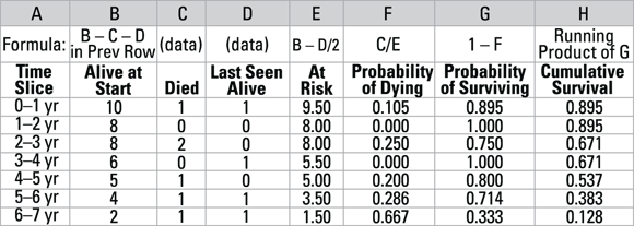
Figure 21-4 shows the spreadsheet with the results of all the preceding calculations.
© John Wiley & Sons, Inc.
FIGURE 21-4: Completed life table to analyze the survival times shown in Figure 22-2.
Interpreting a life table
Figure 21-4 contains the hazard rates (in Column F) and the cumulative survival probabilities (in Column H) for each year following surgery, based on your sample of ten participants. Keep in mind these life-table features:
- The hazard and survival values obtained from this life table are estimates from a sample of the true population hazard and survival functions (in this case, using one-year intervals).
- The intervals are often the same size for all the rows in a life table like in the example, but they don’t have to be. You may choose these on the basis of the probabilities in your data.
- The hazard rate obtained from a life table for each time slice is equal to the Probability of Dying (Column F) divided by the width of the slice. Therefore, the hazard rate for the first year would be expressed as 0.105 per year, or 10.5 percent per year.
- The Cumulative Survival probability, in Column H, is the probability of surviving from the start date through to the end of the interval. It has no units, and it can be expressed as a fraction or as a percentage. The value for any time slice applies to the moment in time at the end of the interval.
- The cumulative survival probability is always 1.0 (or 100 percent) at time 0, whenever you designate that time 0 is (in the example, date of surgery), but it’s not included in the table.
- The cumulative survival function decreases only at the end of an interval that has at least one observed death, because censored observations don’t cause a decrease in the estimated survival. Censored observations however influence the size of the decreases when subsequent events occur. This is because censoring reduces the number at risk, which is used in the denominator in the calculation of the death and survival probabilities.
- If an interval contains no events and no censoring, like in the 1–2 years row in the table in Figure 21-4, it has no impact on the calculations. Notice how all subsequent values for Column B and for Columns E through H would remain identical if that row were removed.
Graphing hazard rates and survival probabilities from a life table
Graphs of hazard rates and cumulative survival probabilities (Columns F and H from Figure 21-4, respectively) can be prepared from life-table results using Microsoft Excel or another spreadsheet or statistical program with graphing capabilities. Figure 21-5 illustrates the way these results are typically presented.
- Figure 21-5a is a graph of hazard rates. Hazard rates are often graphed as bar charts, because each time slice has its own hazard rate in a life table.
- Figure 21-5b is a graph of cumulative survival probabilities, also known as the survival function. Survival values are usually graphed as stepped line charts, where a horizontal line represents the cumulative survival probability during each time slice. The cumulative survival for the Year 0 to 1 time slice is 1.0 (100 percent), so the horizontal line stays at y = 1.0. But between Year 1 and Year 3, the cumulative survival probability drops to 0.895, so a vertical line is dropped from 1.0 to y = 0.895 at the time the Year 1 to Year 2 interval starts. It goes across both that interval and the next one because there are no deaths in these intervals. This stepped line continues downstairs and finally ends at the end of the last interval where the cumulative survival probability is 0.128.

© John Wiley & Sons, Inc.
FIGURE 21-5: Hazard function (a) and survival function (b) results from life-table calculations.
Digging Deeper with the Kaplan-Meier Method
Using very narrow time slices doesn’t hurt life-table calculations. In fact, you can define slices so narrow that each participant’s survival time falls within its own private little slice. Imagine you had N participants. Your life table would have N rows with data from one participant each. You could theoretically add all rest of the rows to fill out the rest of the time slices. These would not have any data in them, and since empty rows don’t affect the life-table calculations, you could just stick with your life table where each row has one participant’s data. And if you happen to have two or more participants with exactly the same survival or censoring time, it’s okay to put each one in their own row.
The life-table calculations work fine with only one participant per row and produce what’s called Kaplan-Meier (K-M) survival estimates. You can think of the K-M method as a very fine-grained life table. Or, you can see a life table as a grouped K-M calculation.
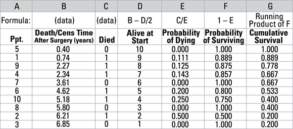
A K-M worksheet for the survival times is shown in Figure 21-6. It is based on the one-participant-per-row idea and is laid out much like the usual life-table worksheet shown in Figure 22-4, but with a few differences in the raw data cells and minor differences in the calculations:
- Instead of a column identifying the time slices, there are two columns identifying the individual participant (Column A) and their survival or censoring time (Column B). The table is ordered from the shortest time to the longest.
- Instead of two columns containing the number who died and were censored in each interval, you need only one column indicating whether or not the participant in that row died (Column C). If they died during the observation period, use code 1, and if not and they were censored, use code 0.
- These changes mean that Column D labeled Alive at Start now decreases by 1 for each subsequent row.
- The At Risk column in Figure 21-4 isn’t needed, because it can be calculated from the Alive at Start column. That’s because if the participant is censored, the probability of dying is calculated as 0, regardless of the value of the denominator.
- To calculate Column E, the Probability of Dying, divide the Died indicator by the number of participants alive for that time period in Column D, Alive at Start. Formula: E = C/D.
- The probability of surviving (Column F) and the cumulative survival (Column G) are calculated the same way as in the life-table method.
© John Wiley & Sons, Inc.
FIGURE 21-6: Kaplan-Meier calculations.
Figure 21-7 shows graphs of the K-M hazard and survival estimates from Figure 21-6. These charts were created using the R statistical software. Most software that performs survival analysis can create graphs similar to this. The K-M survival curve in Figure 21-7b has smaller steps than the life-table survival curve in Figure 21-5b, so it’s more fine-grained. This is because the step curve now decreases at every time point at which a participant died. You can tell from the figures where participant #1 died at 0.74 years, #9 died at 2.27 years, #4 died at 2.34 years, and so on.

© John Wiley & Sons, Inc.
FIGURE 21-7: Kaplan-Meier estimates of the hazard (a) and survival (b) functions.
While the K-M survival curve tends to be smoother than the life table survival curve, just the opposite is true for the hazard curve. In Figure 21-7a, each participant has their own very thin bar, and the resulting chart isn’t easy to interpret.
Heeding a Few Guidelines for Life-Tables and the Kaplan-Meier Method
Most of the larger statistical packages (see Chapter 4) can perform life-table and Kaplan-Meier calculations for you and directly generate survival curves. You have to identify two variables for the software: one with the survival time for each participant, and a binary variable coded 1 if the survival time represents time to death or the event, and 0 if it represents censored time. It sounds simple, but it’s surprisingly easy to mess up. Here are some pointers for setting up your data and interpreting the results properly.
Recording survival times correctly
It is important to draw a distinction between data collection and data analysis. When recording the raw data, it’s best to collect all the relevant dates for the study. Before the study starts, the dates of interest for data collection should be specified, which could include date of diagnosis, start of therapy, end of therapy, start of improvement or remission, date of relapse, or others. For events, you should record date of each event if it recurs, and even if death is not the event of interest, date of death should be recorded if available. For censoring purposes, ensure that you are collecting dates of contact so you can identify a last-seen date if needed. If you collect your data properly, you will later be able to calculate any time interval needed, as well as create an event status indicator needed.
Dates and times should be recorded to suitable precision. If your study timeline is years, it’s best to keep track of dates to the day. In a Phase I clinical trial (see Chapter 5), participants may be studied for events that happen in a span of a few days. In those cases, it’s important to record dates and times to the nearest hour or minute. You can even envision laboratory studies of intracellular events where time would have to be recorded with millisecond — or even microsecond — precision!
 Dates and times can be stored in different ways in different statistical software (as well as Microsoft Excel). Designating columns as being in date format or time format can allow you to perform calendar arithmetic, allowing you to obtain time intervals by subtracting one date from another.
Miscoding censoring information
It can be surprisingly easy to miscode the event status indicator. If the name of the variable is Death, and is coded as 1 if the participant died during the observation period and 0 if they were censored, this seems intuitive. But analysts may want to identify all the censored observations in their data, so they may create a censored indicator named Censored, and code it as 1 if the participant is censored, and 0 if they are not. Because data may be used for different types of survival analyses, there could be other event indicators included in the data as well also coded as 1 and 0.
The problem is that if you accidentally use your censored indicator instead of your event indicator when running your survival analysis, you will unknowingly flip your analysis, and you won’t get any warning or error message from the program. You’ll only get incorrect results. Worse, depending on how many censored and uncensored observations you have, the survival curve may also not hint at any errors. It may look like a perfectly reasonable survival curve for your data, even though it’s completely wrong.
You have to read your software’s documentation carefully to make sure you code your event variable correctly. Also, you should always check the program’s output for the number of censored and uncensored observations and compare them to the known count of censored and uncensored participants in your data file.